Alterative Formulations of Möbius Transformations
Motivation
Möbius Transformations are, in some sense, the analogue of linear transformations in complex analysis. These serve as a really nice entry-point into the behavior of complex functions. They motivate why we should define the point-at-infinity, introduces the Riemann sphere and circle inversion, and provide a simple toy example of a conformal map.
There are many good resources on Möbius transformations. Ch 3.3-3.5 Ahlfors el al., 1979 is the OG text on the subject. For a more modern, lecture-style which emphasizes the analysis, I recommend Michael Penn’s video. For a 3B1B style with nice visualizations, I recommend Mathemaniac’s video. Lastly, I highly recommend this video; short and sweet but highly informative.
In this post, I’m not going to rederive every fact about Möbius transformations (especially when there are already fantastic resources above). Instead, I want to talk about two alternative perspective of Möbius transformations with interesting geometric properties.
A Brief Background
The Extended Complex Plane
We define the extended complex plane as the complex plane augmented with the point-at-infinity, i.e. \(\mathbb{C}^* = \mathbb{C} \cup \{ \infty \}\). It’s important to note that there is no distinction between $+\infty$ and $-\infty$. All lines eventually meet at the point-at-infinity. This may seem strange at first, but the complex plane is more ubiquitously described as the surface of a sphere rather than a flat 2D plane. By adding this extra point-at-infinity, the extended complex plane is now bijective to the Riemann sphere through stereographic projection.
Möbius Transformations
Let $a, b, c, d \in \mathbb{C}$ such that $ad - bc \neq 0$. A Möbius Transformations (also called a fractional linear transformation) is defined as a function $T: \mathbb{C}^* \rightarrow \mathbb{C}^*$ on the extended complex plane such that
\[T(z) = \begin{cases} \frac{a}{c} \qquad &\text{if } z = \infty \\ \infty \qquad &\text{if } z = -\frac{d}{c} \\ \dfrac{az + b}{cz + d} \qquad &\text{otherwise} \end{cases}\]I’ll refer to this as the standard Möbius form. The condition that $ad - bc \neq 0$ ensures that $T$ is invertible (similar to $2\text{D}$ linear algebra) and always differentiable.
I liken the standard Möbius form to the standard form for the equation of a line $Ax + By = C$. While this uniquely defines a line perfectly well, it’s not really all the useful since the parameters $A$, $B$, and $C$ don’t have any geometric meaning. This is why slope-intercept form $y = mx + b$ and point-slope form $y - y_0 = m(x - x_0)$ are preferred and more widely used.
In the remaining of the post I will discuss two alternative formulations which have strong geometric meanings. Note that typically Möbius transformations are reformulated in terms of the cross ratio (see appendix for definition). However, since this is so widely discussed by the resources I provided above, I will not discuss it here.
Steiner Net Form
Consider how a Möbius transformation $S$ transforms the following grid-lines.
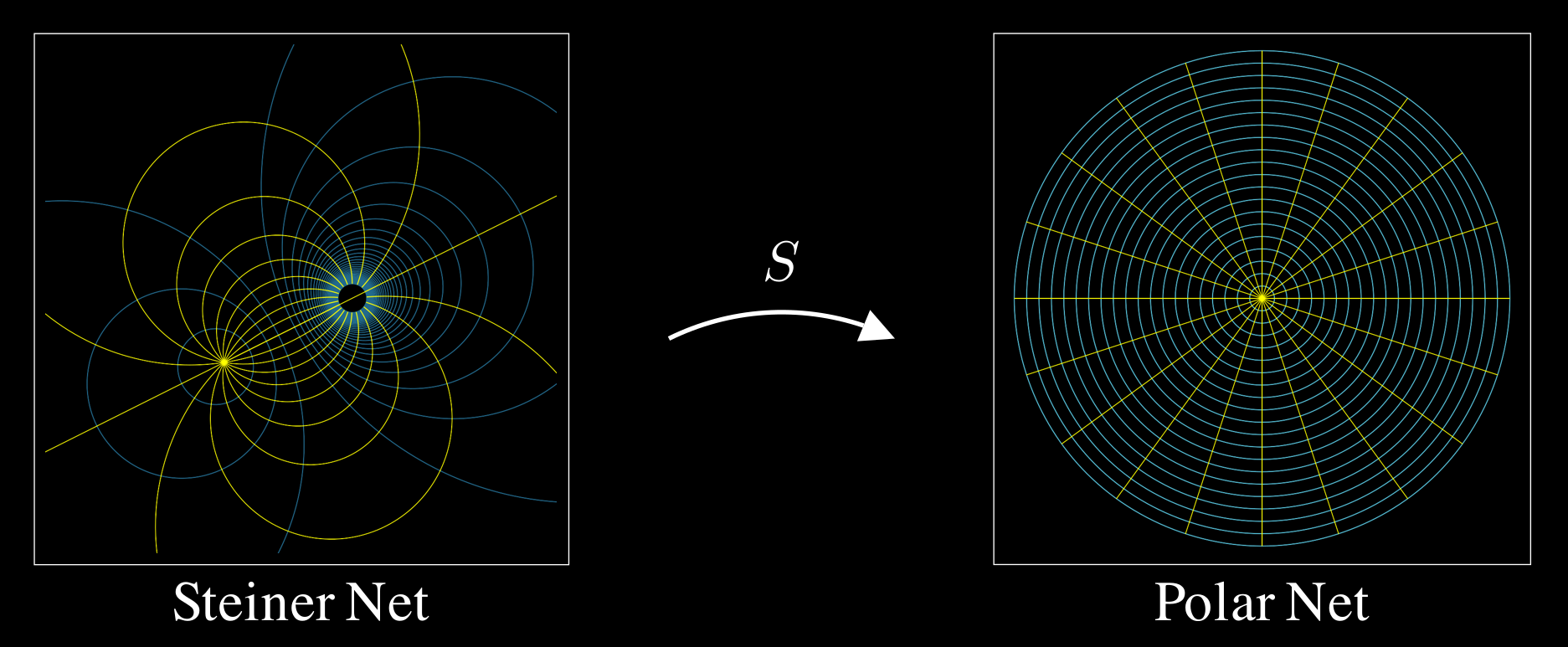
The right-hand image is called a polar net and the left-hand image is called the Steiner net. Applying $S$ transforms the Steiner net into the polar net. Conversely, the inverse of $S$ transforms the polar net into the Steiner net.
To explain the Steiner net, consider the following reformulation.
\[w = \frac{az + b}{cz + d} \ = \ \frac{a}{c} \cdot \frac{z + \frac{b}{a}}{z + \frac{d}{c}} \ \equiv \ k \dfrac{z - p_{0}}{z - p_{\infty}}\]I call this the Steiner Net Form of a Möbius transformation. Notice that $S(p_0) = 0$ and $S(p_{\infty}) = \infty$. So, the center of the polar net moves to $p_0$ in the Steiner net (the very yellow region), and the point-at-infinity of the polar net moves to $p_{\infty}$ in the Steiner net (the black hole looking region).
To understand the affect of $k$, recall the geometric interpretation of complex multiplication; magnitudes multiply and angle add. Thus, the polar net will be scaled by a factor of $\abs{k}$ and rotated through an angle of $\arg k$. In the resulting Steiner net, the blue grid lines scale as $\abs{k}$ scales; the yellow grid lines cycle as $\arg k$ cycles from $0$ to $2\pi$.
To see these geometric properties in action, I’ve created a fun animation.
If you watched the animation, you’ll notice that Steiner nets all essentially look the same, and all you are doing is shifting/scaling them depending on the values of $p_0$, $p_{\infty}$, and $k$. This is a really powerful tool to have if you want to construct a particular Möbius transformation.
You’ll notice a sort of rigidity to the transformation (especially if you watch the animation). If you zoom into a small region of the steiner net, it looks like standard grid-lines again. This characteristic in complex analysis is called conformality, which has a lot of cool properties and I encourage you to look into deeper on your own.
Fixed Point Form
An another perspective is to understand Möbius Transformations through its fixed points. This is arguably less elegant than the Steiner Net interpretation, but has some nice properties.
Proposition: Möbius transformations are uniquely defined by their mapping of $3$ distinct coordinates. Written precisely, given distinct inputs \(z_1, z_2, z_3 \in \mathbb{C}^*\) and distinct outputs \(w_1, w_2, w_3 \in \mathbb{C}^*\) there exists a unique Möbius transformation $T$ such that $T(z_1) = w_1$, $T(z_2) = w_2$, and $T(z_3) = w_3$.
A proof will be provided in the appendix of this post as this is a foundational fact about Möbius transformations, and it is covered by many other sources.
A fixed point of a transformation $T$ is a complex number $z_0$ such that $T(z_0) = z_0$. In particular, for a Möbius transformation
\[z_0 = \frac{az_0 + b}{cz_0 + d} \qquad \implies \qquad cz_0^2 - (a - d)z_0 - b = 0 \qquad \implies \qquad z_0^2 - \left(\tfrac{a - d}{c} \right)z_0 - \tfrac{b}{c} = 0\]Calculating the Fixed Points of a Möbius Transformation
Since Möbius transformations are uniquely defined by their mapping of $3$ distinct coordinates, we can break up the fixed-point analysis into three cases. We are going to do them in reverse order.
Case 3: Three Fixed Points
Suppose there exists distinct \(z_1, z_2, z_3 \in \mathbb{C}^*\) such that $T(z_1) = z_1, \ T(z_2) = z_2, \ \text{and} \ T(z_3) = z_3$.
By the fundamental theorem of algebra, $cz^2 - (a - d)z - b = 0$ can have at most $2$ solutions. Therefore, in order to have three fixed points this expression must be true for all $z$. Thus, $b = c = 0$ and $a = d$ (which would reduce the equation to $0 = 0$), which means $T(z) = z$, i.e. $T$ is the identity transformation.
So, the only Möbius transformations with more than $2$ fixed points is the identity transformation $T(z) = z$, where every point is a fixed point.
Case 2: Two Fixed Points
Applying the quadratic formula to $cz^2 - (a - d)z - b = 0$ gives the following.
\[p_1, p_2 = \frac{(a - d) \pm \sqrt{(a-d)^2 + 4bc}}{2c} \qquad \text{s.t.} \quad (a-d)^2 + 4bc \neq 0\]Additionally, since $0 = (z - p_1)(z - p_2) = z^2 - (p_1 + p_2)z + p_1p_2$, we can equate this to the terms in $0 = z^2 - \left(\frac{a - d}{c} \right)z - \frac{b}{c}$ to get the following properties.
\[p_1 + p_2 = \frac{a - d}{c} \qquad\qquad p_1 \cdot p_2 = - \frac{b}{c}\]Case 1: One Fixed Point
Apply the same method as case 2, except let $(a-d)^2 + 4bc = 0$. Thus,
\[p = \frac{a - d}{2c}\]Notice that
\[2p = \frac{a - d}{c} \qquad\qquad p^2 = - \frac{b}{c}\]is exactly the same as case 2.
Case 0: Zero Fixed Points
This is actually not possible, evident by that the fact that $cz^2 - (a - d)z - b = 0$ always has at least 1 solution in the complex domain. One may object that $T(z) = z + b$ doesn’t have any fixed points. However, $T(\infty) = \infty$ and therefore $\infty$ is the fixed point. And sure enough, you would arrive at this answer by applying the formula from case 1 ($c = 0$).
Another objection might be that we could define $T(z_1) = w_1, \ T(z_2) = w_2, \ \text{and} \ T(z_3) = w_3$ such that $z_1 \neq w_1, \ z_2 \neq w_2, \ \text{and} \ z_3 \neq w_3$. However, that doesn’t mean there aren’t other coordinates which are fixed points. And in fact, there must be at least 1.
Defining Möbius Transformations by Their Fixed Points
Again, we will do this in the reverse order of cases.
Case 3
As shown above, this implies that $T(z) = z$.
Case 2
A Möbius transformation with two fixed points $p_1$ and $p_2$ and $k \in \mathbb{C}$ and $k \neq 0$ can be expressed by the following formula
\[\dfrac{w - p_1}{w - p_2} = k \dfrac{z - p_1}{z - p_2}\]Notice that this is the composition of two Steiner nets. Let $S(z) = \frac{z - p_1}{z - p_2}$, then the above is equivalent to $S(w) = k S(z)$ or $w = S^{-1}(k S(z))$. Prove for yourself that the inverse of a Steiner net is another Steiner net.
Here is the closed-form conversion between the Fixed Point Form and the standard form (proof in the appendix).
\[\begin{cases} &p_1 = \frac{1}{2c} \left [ (a - d) + \sqrt{(a-d)^2 + 4bc} \right ] \\[10pt] &p_2 = \frac{1}{2c} \left [ (a - d) - \sqrt{(a-d)^2 + 4bc} \right ] \\[10pt] &k = \dfrac{cp_2 + d}{cp_1 + d} = \dfrac{(a + d) - \sqrt{(a-d)^2 + 4bc}}{(a + d) + \sqrt{(a-d)^2 + 4bc}} \end{cases} \qquad\iff\qquad \begin{cases} &\text{fix any value of } c \\[10pt] &a = \frac{c}{1-k}(p_1 - kp_2) \\[10pt] &b = -c p_1 p_2 \\[10pt] &d = - \frac{c}{1-k}(p_2 - kp_1) \\[10pt] \end{cases}\]Case 1
A Möbius transformation with one fixed point $p$ and $k \in \mathbb{C}$ can be expressed by the following
\[\dfrac{1}{w - p} = \dfrac{1}{z - p} + k\]Here is the closed-form conversion between the Fixed Point Form and the standard form (proof in the appendix).
\[\begin{cases} &p = \dfrac{a - d}{2c} \\[10pt] &k = \dfrac{2c}{a + d} \end{cases} \qquad\iff\qquad \begin{cases} &\text{fix any value of } c \\[10pt] &a = \frac{c}{k}(1 + kp) \\[10pt] &b = -c p^2 \\[10pt] &d = - \frac{c}{k}(1 - kp) \\[10pt] \end{cases}\]Geometric Properties of the Fixed Point Form
It’s much easier to show rather than explain in words, so I’ve created another animation showing how different values of $p_1$, $p_2$, $p$, and $k$ change the map. In short, the fixed points act as anchors which the rest of the map must rigidly rotate around. $k$ determines how compressed or expanded the map is relative to the fixed points.
The parameter $k$ also defines a homomorphism between the Möbius transformation and the polar net. When creating my animations, this fixed-point form turned out to create the smoothest transitions. For example, when $p_{\infty} = \infty$ in the Steiner Net form, this has to be treated as a special case and there is not a smooth transition to the typical case.